OpenMM 101

This is a simple example of how to use OpenMM to simulate a simple system of particles. The system consists of two particles connected by a harmonic bond. The particles have masses of 1 and 12 amu, and the bond has a length of 1 angstrom and a force constant of 10 kJ/mol/angstrom^2. The system is simulated at 300 K using a Langevin integrator with a timestep of 2 fs. This example shows four important classes in OpenMM: System, Force, Integrator, Platform,and Context. They are the basic building blocks of using OpenMM to simulate a molecular system.

import openmm as mm
import openmm.app as mm_app
import openmm.unit as unit
import numpy as np
import matplotlib.pyplot as plt

Create a system and add two particles to it

system = mm.System()

system.addParticle(1.0 * unit.amu)
system.addParticle(12.0 * unit.amu)

Add a harmonic bond between the two particles

force = mm.HarmonicBondForce()
force.addBond(0, 1, 1.0 * unit.angstrom, 10 * unit.kilojoule_per_mole / unit.angstrom**2)
system.addForce(force)

Run a simulation of the system. We use a Langevin integrator to simulate the system at a constant temperature of 300 K. Using OpenMM, we can choose to run simulations on different platforms that support different hardware. Here we use the Reference platform, which is the slowest one and is useful for testing and debugging. The CPU platform should be used for running production simulations on a CPU. The CUDA platform uses NVIDIA GPUs and is the fastest one. It should be used for running production simulations on a GPU. Here our system is too small to benefit from GPU acceleration, so we use the Reference platform.

integrator = mm.LangevinMiddleIntegrator(300 * unit.kelvin, 1.0 / unit.picosecond, 0.002 * unit.picosecond)

## request the Reference platform
platform = mm.Platform.getPlatformByName('Reference')

## create a simulation context
context = mm.Context(system, integrator, platform)

## set the initial positions of the particles
positions = np.array([[0.0, 0.0, 0.0], [1.0, 0.0, 0.0]], np.float32) * unit.angstrom
context.setPositions(positions)

Running the simulation involves repeatedly calling the step() method of the integrator. This advances the simulation by a specified number of time steps. As the simulation runs, we can query the state of the system to get information about it. For example, here we record the positions and potential energy of the system every 1000 steps.

## run the simulation
xyz = []
us = []
for i in range(3000):
    ## run 1000 steps of dynamics
    integrator.step(1000)

    ## get the positions and potential energy of the system and record them
    state = context.getState(getEnergy=True, getPositions=True)
    xyz.append(state.getPositions(asNumpy=True).value_in_unit(unit.angstrom))
    u = state.getPotentialEnergy().value_in_unit(unit.kilojoule_per_mole)
    us.append(u)
    if (i + 1) % 100 == 0:
        print(i, f'{u:.3f} kJ/mol')

Now that the simulation is complete, let us analyze the trajectory. We will calculate the distance between the two particles and plot a histogram of the distances and the time series of the distance.

## Now let's analyze the trajectory
xyz = np.array(xyz)

d = np.linalg.norm(xyz[:, 1, :] - xyz[:, 0, :], axis=1)

fig = plt.figure()
plt.clf()
plt.hist(d, bins=20, density=True)
plt.xlabel('Distance (angstrom)')
plt.ylabel('Probability Density')
plt.tight_layout()
plt.savefig('./plots/openmm_101_hist.png')

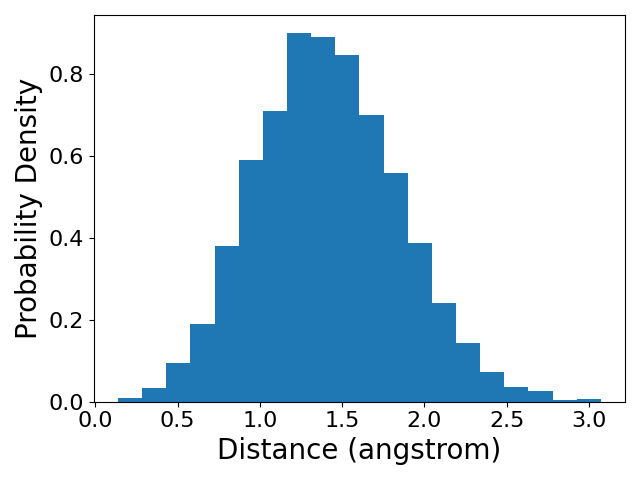
fig = plt.figure()
plt.clf()
plt.plot(d[::10], linewidth=1)
plt.xlabel('Time (ps)')
plt.ylabel('Distance (angstrom)')
plt.tight_layout()
plt.savefig('./plots/openmm_101_timeseries.png')

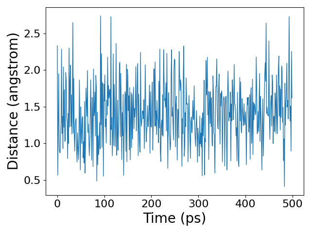
We see that the distance between the two particles fluctuates randomly during the simulation. However, the distribution of distances converges to the equilibrium distribution predicted by the Boltzmann distribution. You could notice that the mean of the distance is not 1 angstrom, which is the equilibrium distance of the harmonic bond. You should think about why this is the case.