Linear Regression using JAX

In this example, we will show how to perform a simple linear regression using JAX. We will generate some synthetic data and fit a linear model to it to recover the true parameters.

import jax
import jax.random as jr
import jax.numpy as jnp
from jax import grad
import matplotlib.pyplot as plt
import jaxopt
jax.config.update("jax_enable_x64", True)

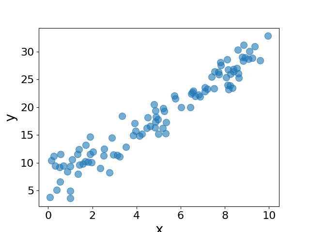
We first generate some synthetic data. We will generate a random number of \(x\) values and compute the corresponding \(y\) values using the equation \(y = k * x + b + \epsilon\), where \(k\) and \(b\) are the true parameters and \(\epsilon\) represents a noise term from a normal distribution.

## prepare synthetic data
key = jr.PRNGKey(10)
subkey, key = jr.split(key)
x = jr.uniform(subkey, shape=(100,), minval=0, maxval=10)

k_true = 2.5
b_true = 5.7
subkey, key = jr.split(key)
y = k_true * x + b_true + jr.normal(subkey, shape=x.shape) * 2.0

fig = plt.figure()
plt.clf()
plt.plot(x, y, "o", alpha = 0.6)
plt.xlabel("x")
plt.ylabel("y")
plt.savefig("./plots/linear_regression_data.png")

If we plot \(y\) against \(x\), we have the following plot:

We will now fit a linear model to the data using the naive gradient descent method. We will define the loss function as the mean squared error between the predicted and true values of \(y\). We will then compute the gradient of the loss function with respect to the parameters \(k\) and \(b\) and update the parameters using the gradient descent algorithm. We will print the loss and the parameters at every 100 steps.

## initial parameters
params = {"k": jnp.zeros(1), "b": jnp.zeros(1)}

def compute_y(params, x):
    k = params["k"]
    b = params["b"]
    return k * x + b

def loss_fn(params, x, y):
    return jnp.mean((compute_y(params, x) - y) ** 2)

grad_fn = grad(loss_fn, argnums=0)

## train the model
lr = 0.01
for i in range(1000):
    grad_params = grad_fn(params, x, y)
    params["k"] -= lr * grad_params["k"]
    params["b"] -= lr * grad_params["b"]
    if i % 100 == 0:
        print(
            f"Loss at step {i:>3}: {loss_fn(params, x, y):>6.2f}, k={params['k'][0]:.2f}, b={params['b'][0]:.2f}"
        )

print("true parameters:")
print(f"k={k_true:>5.2f}, b={b_true:5>.2f}")
print("fitted parameters using naive gradient descent:")
print(f'k={params["k"][0]:>5.2f}, b={params["b"][0]:>5.2f}')

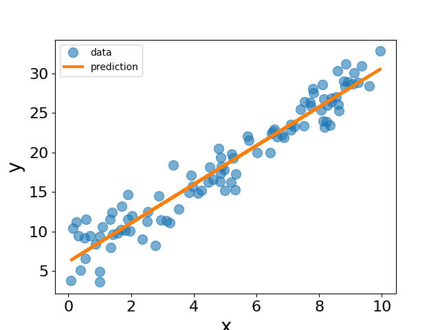
Let us now plot the data and the fitted line using the parameters obtained from the gradient descent algorithm.

y_pred = compute_y(params, x)
fig = plt.figure()
plt.clf()
plt.plot(x, y, "o", label="data", alpha = 0.6)
plt.plot(x, y_pred, label="prediction")
plt.xlabel("x")
plt.ylabel("y")
plt.legend()
plt.savefig("./plots/linear_regression_fit.png")

In real applications, we usually use more sophisticated optimization algorithms to fit the model. Here we will use the LBFGS optimizer from JAXOpt to fit the linear model to the data.

solver = jaxopt.LBFGS(fun=loss_fn, maxiter=100)
init_params = {"k": jnp.zeros(1), "b": jnp.zeros(1)}
res = solver.run(init_params, x=x, y=y)
print("fitted parameters using the LBFGS optimizer")
print(f'k={res.params["k"][0]:>5.2f}, b={res.params["b"][0]:>5.2f}')

We can see that the parameters obtained using the LBFGS optimizer are close to the true parameters. In addition to the LBFGS optimizer, there are many other optimizers available in JAXOpt and other libraries. Different optimizers serve different purposes and may have different convergence properties. It is important to choose the right optimizer for the problem at hand.

The above example is for a linear regression problem with one feature. We can easily extend the example to higher dimensions by generating more features and fitting a linear model to the data. The code below generates a 5-dimensional feature vector and fits a linear model to the data using the LBFGS optimizer.

## higher dimensional
subkey, key = jr.split(key)
X = jr.uniform(subkey, shape=(100, 5), minval=0, maxval=10)
true_k = jnp.array([1.0, 2.0, 3.0, 4.0, 5.0])
true_b = 4.5
subkey, key = jr.split(key)
Y = jnp.dot(X, true_k) + true_b + jr.normal(subkey, shape=(100,)) * 2.0

params = {"k": jnp.zeros(5), "b": jnp.zeros(1)}


def compute_y(params, x):
    k = params["k"]
    b = params["b"]
    return jnp.dot(x, k) + b


def loss_fn(params, x, y):
    return jnp.mean((compute_y(params, x) - y) ** 2)


solver = jaxopt.LBFGS(fun=loss_fn, maxiter=100)
init_params = {"k": jnp.zeros(5), "b": jnp.zeros(1)}
res = solver.run(init_params, x=X, y=Y)
print("true parameters:")
print(f"k={true_k}, b={true_b}")
print("fitted parameters using the LBFGS optimizer:")
print(f'k={res.params["k"]:}, b={res.params["b"][0]:.2f}')