Usage Guide¶

1. When to use the MBAR equations?¶

A common task in computational chemistry is to compute the relative free energies of different thermodynamic states. Suppose there are \(M\) such states, where the \(k\)-th state has a reduced potential energy function \(U_k(x)\) and \(x\) denotes a system conformation. Conformations in the \(k\)-th state follow the Boltzmann distribution \(p_k(x) \propto \exp\left(-U_k(x)\right)\), and the reduced free energy of that state is \(F_k = -\ln \int \exp\left(-U_k(x)\right)\, dx\).

Reduced units

Both \(U_k(x)\) and \(F_k\) are reduced (unitless) quantities that absorb the inverse temperature \(\beta = 1 / k_b T\). If the original potential energy is \(E_k(x)\), then \(U_k(x) = \beta E_k(x)\). To recover a free energy in energy units, multiply the reduced free energy by \(k_b T\), i.e., \(k_b T \, F_k\).

A widely used strategy to obtain the relative free energies of the \(M\) states has two steps:

Sample conformations from each of the \(M\) states separately, using molecular dynamics or Monte Carlo simulations.
Reweight the sampled conformations from all states together to compute the relative free energies.

Let \(N_k\) be the number of conformations sampled from the \(k\)-th state in step 1, denoted \(\{x^{n}_k, \; n = 1, \dots, N_k\}\) for \(k = 1, \dots, M\). The MBAR equations carry out step 2: they reweight these conformations to estimate the relative free energies \(F_k\) for \(k = 1, \dots, M\).

Once solved, the MBAR equations can also estimate the relative free energies of perturbed states from which no conformations were sampled. If there are \(L\) such states, the \(l\)-th perturbed state has its own reduced potential energy function \(U^{\prime}_l(x)\).

This setup is quite general. It covers alchemical free energy calculations as well as computing the potential of mean force (PMF) from umbrella sampling or temperature/Hamiltonian replica exchange simulations.

2. How to use FastMBAR?¶

FastMBAR needs two inputs, both obtained from the sampling above:

an energy matrix \(A\) of the reduced potential energies of the sampled conformations, and
a vector \(v\) holding the number of conformations sampled from each state.

The matrix \(A\) has shape \(M \times N\), where \(M\) is the number of sampled states and \(N = \sum_{k=1}^{M} N_k\) is the total number of conformations from all states. Every conformation is evaluated in all \(M\) states, so each column of \(A\) holds the \(M\) reduced energies of one conformation; that is, \(A_{k,n}\) is the reduced potential energy of the \(n\)-th conformation evaluated in the \(k\)-th state. The vector \(v = (N_1, N_2, \dots, N_M)\) records how many conformations came from each state.

Putting these together, \(A\) is organized as shown below (blue), with its columns grouped by the state each conformation was sampled from. The figure also shows the perturbed energy matrix \(B\) (red), described in the next section.

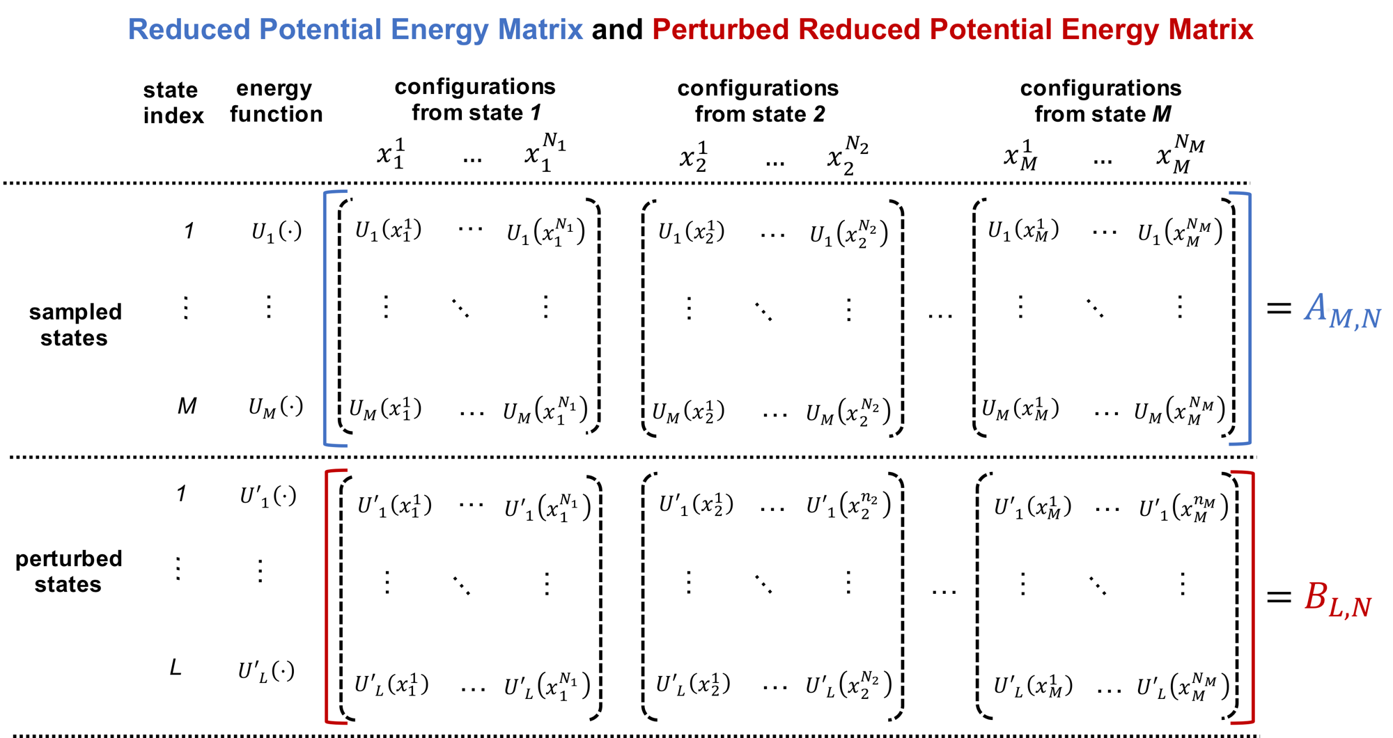
Reduced potential energy matrix A and perturbed reduced potential energy matrix B — The reduced potential energy matrix \(A\) (blue) of the sampled states and the perturbed reduced potential energy matrix \(B\) (red) of the perturbed states. Each column corresponds to one sampled conformation, evaluated in every state.

Reading down a column gives the \(M\) reduced energies of one conformation; reading across a row gives the energies of all \(N\) conformations evaluated in a single state.

Both \(A\) and \(v\) must be NumPy arrays: \(A\) is two-dimensional and \(v\) is one-dimensional. Given them, you create a FastMBAR object, which solves the MBAR equations on construction:

import numpy as np
from bayesmbar import FastMBAR

# construct the energy matrix A and the vector v
...

# initialize FastMBAR; the MBAR equations are solved here
fastmbar = FastMBAR(energy=A, num_conf=v, verbose=True)

# the relative free energies of the M states are stored in fastmbar.F
print(fastmbar.F)

GPU and TPU acceleration

FastMBAR is implemented with JAX and automatically runs on a GPU or TPU when one is available and the matching JAX build is installed. No extra argument is needed to enable it.

To also estimate the uncertainty of the free energies, set bootstrap=True:

import numpy as np
from bayesmbar import FastMBAR

# construct the energy matrix A and the vector v
...

# estimate uncertainties using block bootstrapping
fastmbar = FastMBAR(energy=A, num_conf=v, bootstrap=True, verbose=True)

# free energies and their standard deviations
print(fastmbar.F)
print(fastmbar.F_std)

Column order matters with bootstrapping

When bootstrap=True, the conformations from each state must occupy a contiguous block of columns in \(A\), ordered by state: conformations from state \(k\) must come before those from state \(l\) whenever \(k < l\). When bootstrap=False, the column order does not matter.

Free energies of perturbed states¶

The same FastMBAR object can estimate the relative free energies of perturbed states from which no conformations were sampled. This requires one additional input: a reduced potential energy matrix \(B\).

The matrix \(B\) has shape \(L \times N\), where \(L\) is the number of perturbed states and \(N = \sum_{k=1}^{M} N_k\) is the same total number of conformations sampled from the original \(M\) states. The entry \(B_{l,n}\) is the reduced potential energy of the \(n\)-th conformation evaluated in the \(l\)-th perturbed state. In other words, \(B\) has the same column layout as \(A\), but its rows correspond to the \(L\) perturbed states. \(B\) is shown in red in the figure above, alongside \(A\).

Pass \(B\) to the existing FastMBAR object to compute the perturbed-state free energies:

# compute the relative free energies of the perturbed states
results = fastmbar.calculate_free_energies_of_perturbed_states(B)

# free energies of the perturbed states
print(results["F"])

# their standard deviations
print(results["F_std"])

The returned dictionary also contains DeltaF and DeltaF_std, the pairwise free energy differences between the perturbed states and their standard deviations. See the API reference for details.