Molecular dynamics simulations with OpenMM#
OpenMM is software library for performing molecular dynamics simulations. It is designed to be flexible and efficient and it focuses on simulations of biomolecules. OpenMM is written in C++ and CUDA and has Python bindings, which makes it easy to use in Python scripts. In this example, we will show how to set up molecular dynamics simulations using OpenMM.
[1]:
import openmm as mm
import openmm.app as app
import openmm.unit as unit
import numpy as np
import nglview as nv
import mdtraj
import polars as pl
import matplotlib.pyplot as plt

plt.style.use("seaborn-v0_8-talk")
1. A 1-D harmonic oscillator#
We will start with a simple example of a 1-D harmonic oscillator. In the example, we have a particle of mass 1 amu that is connected to a fixed point by a spring. The particle is constrained to move along the x-axis. The spring has a force constant of 1 kJ/mol/nm^2. The equilibrium position of the particle is at (0, 0, 0), which means the force is zero when the particle is at the origin.
OpenMM uses a class called System to represent the system that we want to simulate. The System class contains a list of particles and a list of forces acting on those particles. To simulate the 1-D harmonic oscillator described above, we need to create a System object for it.
[2]:
## initialize an empty system
system = mm.System()

## add two particles to the system, the first one will be fixed at (0, 0, 0) and the second one
## will be free to move in the x axis. The two particles will be connected by a spring

## add the first particle with mass 0 amu
## OpenMM has a special setting that massless particles are fixed
system.addParticle(0 * unit.amu)

## add the second particle with mass 1 amu
system.addParticle(1 * unit.amu)

print("Number of particles in the system: ", system.getNumParticles())
Number of particles in the system: 2
To model the spring between the two particles, we will add a force between the two particles. The force is given by Hooke’s law: \(f = -kx\), where \(k\) is the force constant and \(x\) is the displacement from the equilibrium position. The potential energy corresponding to this force is given by \(V = \frac{1}{2}kx^2\), which is called the harmonic potential. As a rule of thumb, it is usually easier to specify the potential energy function rather than the force function.
OpenMM has a built-in class called HarmonicBondForce for harmonic potentials.
[3]:
## initialize a HarmonicBondForce
harmonic_force = mm.HarmonicBondForce()

## specify that the force is between the particles with index 0 and 1.
## the index of a particle is the order in which it was added to the system and starts at 0
## because the first particle will be fixed at (0, 0, 0), we set the equilibrium distance to 0 nm
## so that the equilibrium position of the second particle is at (0, 0, 0)
harmonic_force.addBond(
    0, 1, 0.0 * unit.nanometer, 1 * unit.kilojoule_per_mole / unit.nanometer**2
)

## add the force to the system
system.addForce(harmonic_force)
[3]:
0
In OpenMM, each particle has three coordinates \((x, y, z)\). To mimic the constraint of the second particle along the x-axis, we add a large external force on the second particle in the y and z directions. This force is large enough to keep the second particle from moving in the y and z directions. We use `CustomExternalForce <http://docs.openmm.org/latest/api-python/generated/openmm.openmm.CustomExternalForce.html#openmm.openmm.CustomExternalForce>`__ in OpenMM to apply this force. The
CustomExternalForce class allows us to specify a custom force function that can depend on the coordinates of the particles. In this case, we will use a harmonic potential in the y and z directions with a large force constant and the equilibrium position at 0.0. This will create a large force on the second particle in the y and z directions if it moves away from 0 in those directions. It effectively constrains the second particle to move only in the x direction.
[4]:
k_external = 100
external_force = mm.CustomExternalForce("0.5*k_external*(y^2 + z^2)")
external_force.addGlobalParameter("k_external", k_external)
external_force.addParticle(1, [])

system.addForce(external_force)
[4]:
1
To simulate the system, we need to specify the integrator used to integrate the equations of motion. OpenMM has several built-in integrators, including LangevinIntegrator, VerletIntegrator, and BrownianIntegrator. In this example, we will first use the VerletIntegrator to integrate the Hamiltonian equations of motion.
In addition, we also need to specify the kind of hardware we are using to run the simulation. OpenMM can run on a CPU or a GPU and it uses the class Platform to specify the hardware. In this example, we will use the CPU platform to run the simulation on the CPU.
There is one more thing we need to do before we can run the simulation in OpenMM. OpenMM uses a class called Context to represent the complete state of a simulation and a Context object is created from a System object, an Integrator object, and a Platform object. The Context object contains among other things the positions and velocities of all the particles in the
system. Before running the simulation, we also need to set the initial positions and velocities of the particles in the context.
[10]:
## create an integrator with a time step of 0.1 ps
## you could change the size of the time step to see how it affects the simulation
step_size = 0.1
integrator = mm.VerletIntegrator(step_size * unit.picoseconds)

## pick a platform
## in this case we will use the CPU platform
## if you want to use NVIDIA GPU, you could use "CUDA" instead
platform = mm.Platform.getPlatformByName("CPU")

## create a context
context = mm.Context(system, integrator, platform)


## set the initial positions of the particles
init_x = np.array(
    [
        [0.0, 0.0, 0.0],  # particle 0
        [0.0, 0.0, 0.0],  # particle 1
    ]
)

context.setPositions(init_x)

## set the initial velocities of the particles
init_v = np.array(
    [
        [0.0, 0.0, 0.0],  # particle 0
        [1.0, 0.0, 0.0],  # particle 1
    ]
)

context.setVelocities(init_v)

## because the initial velocity of the second particle is (1, 0, 0) and its initial position
## is at the equilibrium position of the spring, the total energy of the second particle is
## 0.5 * m * v^2 = 0.5 * 1 * 1^2 = 0.5
Now we are ready to run the simulation. To take a time step in the simulation, we call the step method of the integrator. After taking a time step, we record the new positions and velocities of the particles from the context.
[11]:
xs = []  # positions
vs = []  # velocities
us = []  # potential energy
ks = []  # kinetic energy
es = []  # total energy

for i in range(50):
    integrator.step(1)

    state = context.getState(getEnergy=True, getPositions=True, getVelocities=True)
    x = state.getPositions(asNumpy=True).value_in_unit(unit.nanometer)
    v = state.getVelocities(asNumpy=True).value_in_unit(
        unit.nanometer / unit.picosecond
    )
    u = state.getPotentialEnergy().value_in_unit(unit.kilojoule_per_mole)
    k = state.getKineticEnergy().value_in_unit(unit.kilojoule_per_mole)

    xs.append(x)
    vs.append(v)
    us.append(u)
    ks.append(k)
    es.append(u + k)

    print(
        f"step: {i + 1:3d};  u: {u:6.3f}; x: {x[1][0]:6.3f}; k: {k:6.3f}; v: {v[1][0]:6.3f}; e: {u + k:6.3f}"
    )

xs = np.array(xs)
vs = np.array(vs)
us = np.array(us)
ks = np.array(ks)
step:   1;  u:  0.005; x:  0.100; k:  0.495; v:  1.000; e:  0.500
step:   2;  u:  0.020; x:  0.199; k:  0.480; v:  0.990; e:  0.500
step:   3;  u:  0.044; x:  0.296; k:  0.456; v:  0.970; e:  0.500
step:   4;  u:  0.076; x:  0.390; k:  0.424; v:  0.940; e:  0.500
step:   5;  u:  0.115; x:  0.480; k:  0.385; v:  0.901; e:  0.500
step:   6;  u:  0.160; x:  0.566; k:  0.340; v:  0.853; e:  0.500
step:   7;  u:  0.208; x:  0.645; k:  0.292; v:  0.797; e:  0.501
step:   8;  u:  0.258; x:  0.718; k:  0.243; v:  0.732; e:  0.501
step:   9;  u:  0.308; x:  0.785; k:  0.193; v:  0.661; e:  0.501
step:  10;  u:  0.355; x:  0.843; k:  0.146; v:  0.582; e:  0.501
step:  11;  u:  0.398; x:  0.893; k:  0.103; v:  0.498; e:  0.501
step:  12;  u:  0.436; x:  0.933; k:  0.065; v:  0.409; e:  0.501
step:  13;  u:  0.466; x:  0.965; k:  0.036; v:  0.315; e:  0.501
step:  14;  u:  0.487; x:  0.987; k:  0.014; v:  0.219; e:  0.501
step:  15;  u:  0.499; x:  0.999; k:  0.002; v:  0.120; e:  0.501
step:  16;  u:  0.501; x:  1.001; k:  0.000; v:  0.020; e:  0.501
step:  17;  u:  0.493; x:  0.993; k:  0.008; v: -0.080; e:  0.501
step:  18;  u:  0.475; x:  0.975; k:  0.026; v: -0.179; e:  0.501
step:  19;  u:  0.449; x:  0.947; k:  0.053; v: -0.277; e:  0.501
step:  20;  u:  0.414; x:  0.910; k:  0.087; v: -0.371; e:  0.501
step:  21;  u:  0.373; x:  0.864; k:  0.128; v: -0.462; e:  0.501
step:  22;  u:  0.327; x:  0.809; k:  0.174; v: -0.549; e:  0.501
step:  23;  u:  0.278; x:  0.746; k:  0.222; v: -0.630; e:  0.501
step:  24;  u:  0.228; x:  0.676; k:  0.272; v: -0.704; e:  0.501
step:  25;  u:  0.179; x:  0.598; k:  0.321; v: -0.772; e:  0.500
step:  26;  u:  0.133; x:  0.515; k:  0.368; v: -0.832; e:  0.500
step:  27;  u:  0.091; x:  0.427; k:  0.409; v: -0.883; e:  0.500
step:  28;  u:  0.056; x:  0.334; k:  0.444; v: -0.926; e:  0.500
step:  29;  u:  0.028; x:  0.238; k:  0.472; v: -0.959; e:  0.500
step:  30;  u:  0.010; x:  0.140; k:  0.490; v: -0.983; e:  0.500
step:  31;  u:  0.001; x:  0.040; k:  0.499; v: -0.997; e:  0.500
step:  32;  u:  0.002; x: -0.060; k:  0.498; v: -1.001; e:  0.500
step:  33;  u:  0.013; x: -0.159; k:  0.487; v: -0.995; e:  0.500
step:  34;  u:  0.033; x: -0.257; k:  0.467; v: -0.979; e:  0.500
step:  35;  u:  0.062; x: -0.353; k:  0.438; v: -0.954; e:  0.500
step:  36;  u:  0.099; x: -0.444; k:  0.401; v: -0.918; e:  0.500
step:  37;  u:  0.141; x: -0.532; k:  0.359; v: -0.874; e:  0.500
step:  38;  u:  0.188; x: -0.614; k:  0.312; v: -0.821; e:  0.500
step:  39;  u:  0.238; x: -0.690; k:  0.263; v: -0.759; e:  0.501
step:  40;  u:  0.288; x: -0.759; k:  0.213; v: -0.690; e:  0.501
step:  41;  u:  0.336; x: -0.820; k:  0.164; v: -0.614; e:  0.501
step:  42;  u:  0.382; x: -0.874; k:  0.119; v: -0.532; e:  0.501
step:  43;  u:  0.421; x: -0.918; k:  0.080; v: -0.445; e:  0.501
step:  44;  u:  0.454; x: -0.953; k:  0.047; v: -0.353; e:  0.501
step:  45;  u:  0.479; x: -0.979; k:  0.022; v: -0.258; e:  0.501
step:  46;  u:  0.495; x: -0.995; k:  0.006; v: -0.160; e:  0.501
step:  47;  u:  0.501; x: -1.001; k:  0.000; v: -0.060; e:  0.501
step:  48;  u:  0.497; x: -0.997; k:  0.004; v:  0.040; e:  0.501
step:  49;  u:  0.483; x: -0.983; k:  0.018; v:  0.139; e:  0.501
step:  50;  u:  0.460; x: -0.960; k:  0.041; v:  0.238; e:  0.501
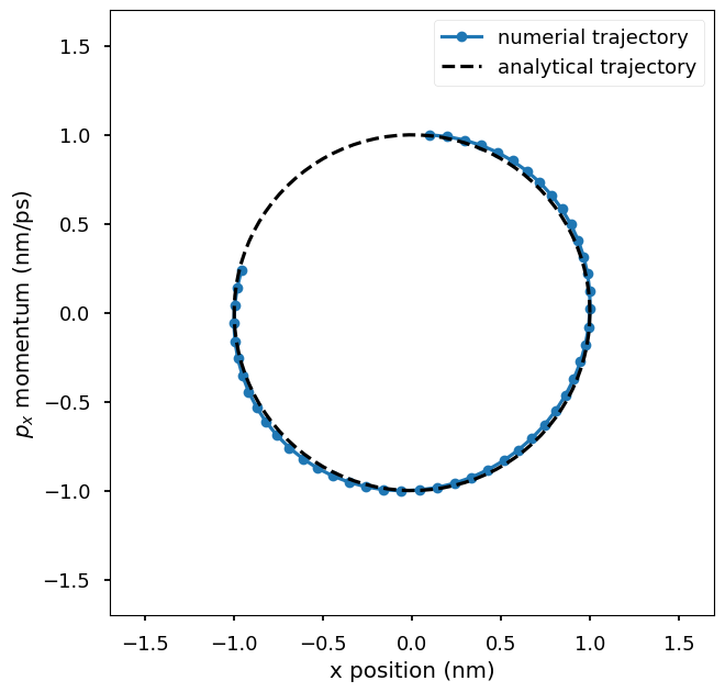
Plot the numerical trajectory in the phase space of \((x, p_x)\) where x is the x-coordinate of the particle and p_x is the x-component of the momentum of the particle. The numerical trajectory is compared to the analytical trajectory. You could change the step size used in the integrator to see how it affects the accuracy of the numerical trajectory.
[12]:
ps = vs  ## momentum
plt.plot(xs[:, 1, 0], ps[:, 1, 0], "o-", label="numerial trajectory", markersize=7)
plt.plot(
    np.cos(np.linspace(0, 2 * np.pi, 100)),
    np.sin(np.linspace(0, 2 * np.pi, 100)),
    "k--",
    label="analytical trajectory",
)
plt.xlim(-1.7, 1.7)
plt.ylim(-1.7, 1.7)
plt.xlabel("x position (nm)")
plt.ylabel(r"$p_x$ momentum (nm/ps)")
plt.legend()
plt.gca().set_aspect("equal", adjustable="box")
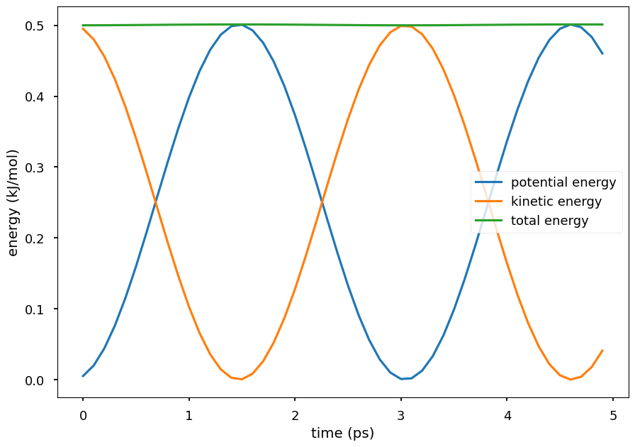
Plot the potential energy and kinetic energy of the particle as a function of time. The Hamiltonian equation of motion is energy conserving, so the total energy of the system is close to a constant. The small oscillations in the total energy are due to numerical errors in the integration. The kinetic energy and potential energy oscillate in time. Because the Hamiltonian equations is energy conserving, conformations sampled by integrating the Hamiltonian equations are the ones from the system’s NVE ensemble.
[13]:
plt.plot(np.arange(len(us)) * step_size, us, label="potential energy")
plt.plot(np.arange(len(ks)) * step_size, ks, label="kinetic energy")
plt.plot(np.arange(len(us)) * step_size, us + ks, label="total energy")
plt.xlabel("time (ps)")
plt.ylabel("energy (kJ/mol)")
plt.legend()
plt.show()
To sample from the NVT ensemble, we can use the LangevinIntegrator instead of the VerletIntegrator. The Langevin integrator integrates the Langevin equations of motion, which mathematically models the effect of a heat bath on the system.
[30]:
## construct a Langevin integrator at temperature T
T = 300
integrator = mm.LangevinIntegrator(
    T * unit.kelvin,  # temperature
    1 / unit.picosecond,  # friction coefficient
    step_size * unit.picoseconds,  # time step
)

platform = mm.Platform.getPlatformByName("CPU")

context = mm.Context(system, integrator, platform)
context.setPositions(init_x)
context.setVelocitiesToTemperature(T)

xs = []  # positions
vs = []  # velocities
us = []  # potential energy
ks = []  # kinetic energy
es = []  # total energy

for i in range(5000):
    integrator.step(1)

    state = context.getState(getEnergy=True, getPositions=True, getVelocities=True)
    x = state.getPositions(asNumpy=True).value_in_unit(unit.nanometer)
    v = state.getVelocities(asNumpy=True).value_in_unit(
        unit.nanometer / unit.picosecond
    )
    u = state.getPotentialEnergy().value_in_unit(unit.kilojoule_per_mole)
    k = state.getKineticEnergy().value_in_unit(unit.kilojoule_per_mole)

    xs.append(x)
    vs.append(v)
    us.append(u)
    ks.append(k)
    es.append(u + k)

    if (i + 1) % 100 == 0:
        print(
            f"step: {i + 1:3d};  u: {u:6.3f}; x: {x[1][0]:6.3f}; k: {k:6.3f}; v: {v[1][0]:6.3f}; e: {u + k:6.3f}"
        )

xs = np.array(xs)
vs = np.array(vs)
us = np.array(us)
ks = np.array(ks)
ps = vs  ## momentum
step: 100;  u:  3.136; x:  1.143; k:  4.316; v: -1.446; e:  7.452
step: 200;  u:  5.647; x: -0.147; k:  2.820; v:  1.977; e:  8.467
step: 300;  u:  0.340; x:  0.822; k:  2.614; v: -1.473; e:  2.954
step: 400;  u:  4.014; x:  2.009; k:  2.485; v: -1.167; e:  6.499
step: 500;  u:  5.025; x:  1.706; k:  2.618; v: -1.262; e:  7.644
step: 600;  u:  6.007; x: -2.908; k: 10.900; v: -0.102; e: 16.907
step: 700;  u:  6.871; x: -2.736; k:  1.911; v: -1.451; e:  8.782
step: 800;  u:  5.153; x: -0.937; k:  0.569; v: -1.015; e:  5.722
step: 900;  u: 11.561; x: -3.538; k:  2.376; v:  0.843; e: 13.937
step: 1000;  u:  3.798; x:  0.118; k:  0.044; v: -0.211; e:  3.842
step: 1100;  u:  1.162; x: -0.731; k:  1.781; v: -1.721; e:  2.943
step: 1200;  u:  3.194; x: -0.520; k:  2.819; v: -0.149; e:  6.013
step: 1300;  u:  2.521; x:  0.717; k:  0.610; v: -0.550; e:  3.130
step: 1400;  u:  0.744; x:  1.014; k:  9.965; v:  2.138; e: 10.709
step: 1500;  u:  5.642; x:  0.674; k:  6.134; v:  2.863; e: 11.776
step: 1600;  u:  6.841; x: -3.614; k:  2.219; v: -0.808; e:  9.060
step: 1700;  u:  3.040; x:  1.344; k:  3.664; v:  0.673; e:  6.704
step: 1800;  u:  2.067; x: -1.697; k:  0.803; v:  1.038; e:  2.870
step: 1900;  u:  2.889; x:  0.635; k: 12.177; v: -0.983; e: 15.066
step: 2000;  u:  8.295; x: -2.194; k:  1.198; v: -1.219; e:  9.494
step: 2100;  u:  8.324; x: -3.638; k: 10.878; v: -3.511; e: 19.201
step: 2200;  u:  3.865; x:  1.409; k:  5.397; v:  1.929; e:  9.262
step: 2300;  u:  1.330; x:  0.760; k:  4.454; v: -1.262; e:  5.784
step: 2400;  u:  2.513; x:  0.182; k:  1.250; v: -0.228; e:  3.763
step: 2500;  u:  2.130; x:  1.796; k:  1.418; v:  0.883; e:  3.548
step: 2600;  u:  1.078; x: -1.465; k:  5.116; v:  1.153; e:  6.193
step: 2700;  u:  2.889; x: -1.306; k:  2.660; v: -1.008; e:  5.549
step: 2800;  u:  0.061; x: -0.169; k:  0.144; v: -0.273; e:  0.205
step: 2900;  u:  4.533; x:  0.894; k:  7.148; v: -2.709; e: 11.681
step: 3000;  u:  3.791; x: -2.451; k:  1.228; v:  1.200; e:  5.019
step: 3100;  u:  4.831; x: -2.756; k:  0.890; v:  1.092; e:  5.720
step: 3200;  u:  5.473; x: -1.959; k:  9.813; v:  2.866; e: 15.286
step: 3300;  u:  7.220; x: -2.735; k:  1.556; v:  0.022; e:  8.776
step: 3400;  u:  6.623; x: -0.561; k:  5.976; v:  2.070; e: 12.598
step: 3500;  u:  6.757; x: -0.610; k:  1.035; v:  0.264; e:  7.792
step: 3600;  u:  0.550; x: -0.413; k:  5.680; v: -2.720; e:  6.231
step: 3700;  u:  1.692; x:  0.489; k:  0.447; v:  0.653; e:  2.139
step: 3800;  u:  6.270; x: -1.250; k:  2.067; v:  0.655; e:  8.337
step: 3900;  u:  6.321; x: -2.097; k:  9.159; v:  0.808; e: 15.480
step: 4000;  u:  3.072; x:  1.123; k:  0.240; v:  0.064; e:  3.313
step: 4100;  u:  3.369; x:  0.462; k:  3.320; v:  0.115; e:  6.689
step: 4200;  u: 14.947; x:  0.464; k:  0.889; v:  0.119; e: 15.836
step: 4300;  u:  3.243; x: -0.420; k:  0.818; v: -0.501; e:  4.061
step: 4400;  u:  5.749; x:  2.815; k:  3.271; v: -0.253; e:  9.021
step: 4500;  u:  0.198; x: -0.614; k:  1.135; v: -0.438; e:  1.333
step: 4600;  u:  3.195; x: -1.967; k:  2.052; v: -1.900; e:  5.247
step: 4700;  u:  4.118; x: -1.258; k:  9.072; v:  1.114; e: 13.190
step: 4800;  u:  0.918; x:  0.572; k:  1.342; v: -0.551; e:  2.260
step: 4900;  u:  9.108; x:  3.819; k:  0.248; v:  0.598; e:  9.356
step: 5000;  u:  2.552; x:  0.068; k:  4.860; v: -0.651; e:  7.412
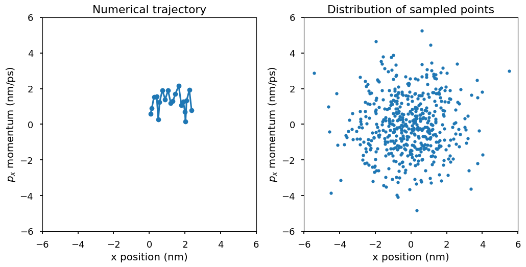
Plot \((x, p_x)\) for the second particle. The first plot shows the numerical trajectory in the first 50 steps. Because the Langevin integrator is a stochastic integrator, the trajectory is stochastic. The second plot shows more \((x, p_x)\) points from the trajectory. In the second plot, a pattern emerges. Those points of \((x, p_x)\) are distributed according to a 2-d Gaussian distribution, which is the Boltzmann distribution at temperature T, i.e., \(p(x, p_x)\) is proportional to \(\exp(-E(x, p_x)/k_BT)\) where \(E(x, p_x) = U(x) + K(p_x) = 1/2kx^2 + 1/2mv^2 = 1/2x^2 + 1/2p_x^2\). The Boltzmann distribution of the system is a 2-d Gaussian distribution with mean \((0, 0)\) and variance \((k_BT, k_BT)\).
[31]:
plt.subplot(1, 2, 1)
plt.plot(xs[:20, 1, 0], ps[:20, 1, 0], "o-", markersize=7)
plt.xlim(-6, 6)
plt.ylim(-6, 6)
plt.gca().set_aspect("equal", adjustable="box")
plt.xlabel("x position (nm)")
plt.ylabel(r"$p_x$ momentum (nm/ps)")
plt.title("Numerical trajectory")

plt.subplot(1, 2, 2)
plt.plot(xs[::10, 1, 0], ps[::10, 1, 0], ".")
plt.xlim(-6, 6)
plt.ylim(-6, 6)
plt.xlabel("x position (nm)")
plt.ylabel(r"$p_x$ momentum (nm/ps)")
plt.gca().set_aspect("equal", adjustable="box")
plt.title("Distribution of sampled points")
plt.tight_layout()
plt.show()
Let compute the mean and variance of the sampled \((x, p_x)\) points and see if they are close to the expected values.
[32]:
print(f"mean of x: {np.mean(xs[::10, 1, 0]):.3f}")
print(f"mean of p_x: {np.mean(ps[::10, 1, 0]):.3f}")

print(f"variance of x: {np.var(xs[::10, 1, 0]):.3f}")
print(f"variance of p_x: {np.var(ps[::10, 1, 0]):.3f}")
mean of x: -0.134
mean of p_x: -0.042
variance of x: 2.616
variance of p_x: 2.695
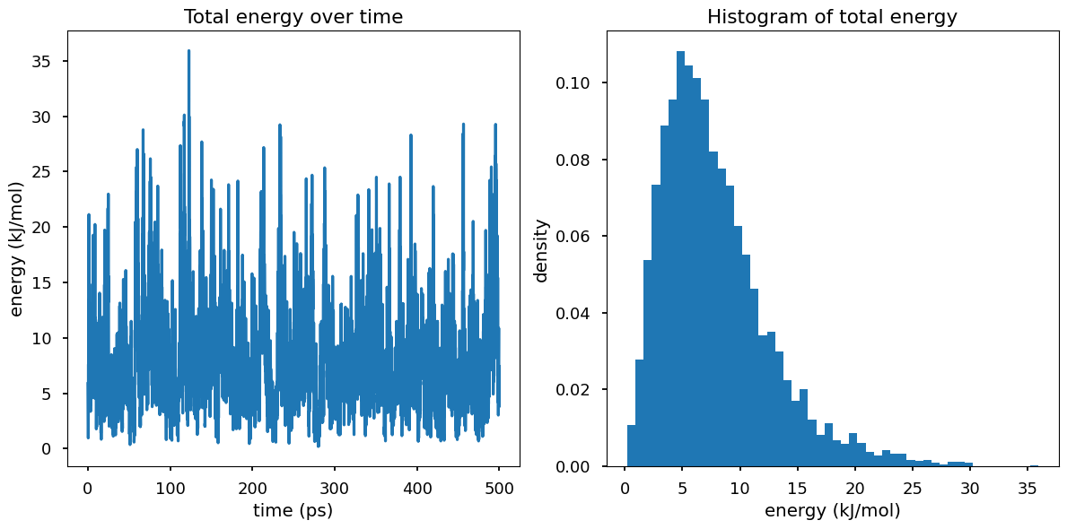
In the NVT ensemble, the system is in contact with a heat bath at temperature T and therefore the system can exchange energy with the heat bath, which results in the fluctuations in the total energy of the system.
[33]:
plt.figure(figsize=(12, 6))
plt.subplot(1, 2, 1)
plt.plot(
    np.arange(len(us)) * step_size,
    es,
    label="total energy",
)
plt.xlabel("time (ps)")
plt.ylabel("energy (kJ/mol)")
plt.title("Total energy over time")

plt.subplot(1, 2, 2)
plt.hist(es, bins=50, density=True)
plt.xlabel("energy (kJ/mol)")
plt.ylabel("density")
plt.title("Histogram of total energy")
plt.tight_layout()
plt.show()
2. A box of water#
In this example, we will simulate a box of water in the NPT ensemble. Similar to the previous example, we will need to create a System object to represent the system. In the previous example, the system is so simple that we can create the System object manually. In this example, the system will involves a lot more particles and the interactions between them are more complicated. Therefore, we will use built-in functions in OpenMM to create the system. The code in the following cell will
create a System object for a box of water. The box is 2nm x 2nm x 2nm. The water molecules are modelled using the TIP3P water model. The TIP3P water model is a simple rigid-body model for water that consists of three particles: two hydrogen atoms and one oxygen atom.
[34]:
## OpenMM provides functions to create a system using a force field and a topology
## a force field is a set of parameters that describe the interactions between different types of particles
## a topology is a description of the connectivity of the particles in the system

## the force field
forcefield = app.ForceField("amber14-all.xml", "amber14/tip3p.xml")

## the topology
top = app.Topology()
pos = np.zeros([0, 3])
mol = app.Modeller(topology=top, positions=pos)
mol.addSolvent(forcefield, model="tip3p", boxSize=(2.5, 2.5, 2.5))
top, pos = mol.getTopology(), mol.getPositions()

## create the system
system = forcefield.createSystem(
    top,
    nonbondedMethod=app.PME,
    nonbondedCutoff=1.0 * unit.nanometers,
    rigidWater=True,
)

## we can save the system to a file
## you could look at the file to see what are included in the system
with open("system.xml", "w") as f:
    f.write(mm.XmlSerializer.serialize(system))
To visualize the system, we will save the coordinates of the particles in the system to a PDB file.
[35]:
## save the pdb file
app.PDBFile.writeFile(top, pos, open("water.pdb", "w"))

## visualize
view = nv.show_structure_file("water.pdb")
view.add_ball_and_stick()
view.center()
view
We can query various information about the system, such as the number of particles, forces acting on the particles, and the periodic box.
[36]:
num_of_particles = system.getNumParticles()
print(f"Number of particles in the system: {num_of_particles}")

## forces in the system
forces = system.getForces()
print(f"Number of forces in the system: {len(forces)}")
names = [force.getName() for force in forces]
print("forces in the system: ", names)
Number of particles in the system: 1503
Number of forces in the system: 5
forces in the system:  ['HarmonicBondForce', 'NonbondedForce', 'PeriodicTorsionForce', 'CMMotionRemover', 'HarmonicAngleForce']
To simulate the system at constant pressure, we will add a MonteCarloBarostat to the system. The MonteCarloBarostat implements the Monte Carlo method to control the pressure of the system. It is classified as a special type of force in OpenMM and it needs to be added to the system as other forces. The MonteCarloBarostat will periodically propose a volume change and accept or reject the volume change using the Metropolis algorithm.
[37]:
system.addForce(mm.MonteCarloBarostat(1 * unit.bar, 300 * unit.kelvin, 25))
print("Forces after adding barostat:")
forces = system.getForces()
print(f"Number of forces in the system: {len(forces)}")
names = [force.getName() for force in forces]
print("forces in the system: ", names)
Forces after adding barostat:
Number of forces in the system: 6
forces in the system:  ['HarmonicBondForce', 'NonbondedForce', 'PeriodicTorsionForce', 'CMMotionRemover', 'HarmonicAngleForce', 'MonteCarloBarostat']
We will use the LangevinIntegrator to control the temperature of the system. Although we could use the Context class for running the simulation, we will use the Simulation class instead. The Simulation class is a higher-level interface for running simulations in OpenMM. It provides a convenient way to set up and run simulations, and it will automatically create a Context object for us.
[38]:
## create a Langevin integrator at temperature T
integrator = mm.LangevinIntegrator(
    298.15 * unit.kelvin,  # temperature
    1 / unit.picosecond,  # friction coefficient
    0.002 * unit.picoseconds,  # time step
)

## pick a platform
platform = mm.Platform.getPlatformByName("CPU")

## create a simulation
## the simulation object will create a context and
simulation = app.Simulation(top, system, integrator, platform)

## set the initial positions of the particles
simulation.context.setPositions(pos)
Minimize the system to remove any bad contacts between the water molecules. When running a simulation with a large number of particles, it is usually a good idea to minimize the system first. The Simulation class has a built-in method for minimizing the energy of the system.
[39]:
state = simulation.context.getState(getEnergy=True)
u = state.getPotentialEnergy().value_in_unit(unit.kilojoule_per_mole)
print(f"potential energy before minimization: {u:.3f} kJ/mol")

simulation.minimizeEnergy()

state = simulation.context.getState(getEnergy=True)
u = state.getPotentialEnergy().value_in_unit(unit.kilojoule_per_mole)
print(f"potential energy after minimization: {u:.3f} kJ/mol")
potential energy before minimization: -1607.764 kJ/mol
potential energy after minimization: -24029.260 kJ/mol
Now we are ready to run the simulation. During the simulation, we will save the trajectory of the system to a DCD file. The DCD file format is a common binary format for storing molecular dynamics trajectories.
[40]:
## set the initial velocities of the particles
simulation.context.setVelocitiesToTemperature(300 * unit.kelvin)

## add a reporter to the simulation
dcd_reporter = app.DCDReporter("water.dcd", 100)
simulation.reporters.append(dcd_reporter)

## add a state reporter to the simulation
state_reporter = app.StateDataReporter(
    "water.csv", 100, step=True, potentialEnergy=True, volume=True, density=True
)
simulation.reporters.append(state_reporter)

## run the simulation for 10 ps
simulation.step(50_000)
It is important to always look at the trajectory of a simulation to rule out any apparent issues.
[41]:
traj = mdtraj.load_dcd("water.dcd", top=mdtraj.Topology.from_openmm(top))
traj_view = nv.show_mdtraj(traj)
traj_view.add_ball_and_stick()
traj_view.center()
traj_view
After obtaining the trajectory, we compute various properties of the system. The following properties are directly available from the state recorded during the simulation.
[42]:
df = pl.read_csv("water.csv")

plt.subplot(3, 1, 1)
plt.plot(df.select(pl.col("Potential Energy (kJ/mole)")), label="Potential Energy")
plt.ylabel("Potential Energy (kJ/mole)")
plt.xlabel("Step")
plt.legend()

plt.subplot(3, 1, 2)
plt.plot(df.select(pl.col("Box Volume (nm^3)")), label="Box Volume")
plt.ylabel("Box Volume (nm^3)")
plt.xlabel("Step")
plt.legend()

plt.subplot(3, 1, 3)
plt.plot(df.select(pl.col("Density (g/mL)")), label="Density")
plt.ylabel("Density (g/mL)")
plt.xlabel("Step")
plt.legend()

plt.tight_layout()
plt.show()
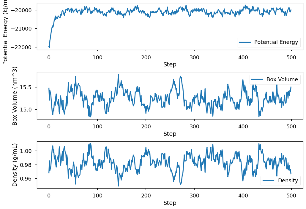
From the plot of the potential energy, we can see that the potential energy first relaxed and then fluctuated around an average value. Because we minimized the system before running the simulation, the system is not in equilibrium yet at the beginning of the simulation. It takes some time for the system to relax to equilibrium, after which the potential energy fluctuates around an average value. When computing equilibrium properties of the system, we need to exclude the part of the trajectory before the system reaches equilibrium. In addition, we saved the conformation for the system every 100 steps, which corresponds to 0.2 ps. Because adjacent conformations are only 0.2 ps apart, they are correlated as shown in all three plots: if the value of the property at time t is high, the value of the property at time t+1 also tends to be high. When computing the average value of the property, we want to use uncorrelated samples. To do this, we use conformations that are separated by a longer time interval.
In the following, we exclude the first 50 snapshots and use every 5th snapshot to compute the average value of the property.
[44]:
df = df[50::5]
[45]:
## density
density = df.select(pl.col("Density (g/mL)")).to_numpy().flatten()
print("=" * 50)
print(f"density from simulation: {np.mean(density):.3f} g/mL")
print("experimental value: 0.997 g/mL")

## average potential energy
u = df.select(pl.col("Potential Energy (kJ/mole)")).to_numpy().flatten()
num_water = system.getNumParticles() // 3
u = u / num_water
u = np.mean(u)
print("=" * 50)
print(f"potential energy per water from simulation: {u:.3f} kJ/mol")
print("experimental value: - 41.505 kJ/mol")

## enthalpy of vaporization
DeltaU = -u
V = df.select(pl.col("Box Volume (nm^3)")).to_numpy().flatten().mean().item()
V_liquid = V / num_water

V_gas = unit.MOLAR_GAS_CONSTANT_R * 298.15 * unit.kelvin / (1 * unit.bar)
V_gas = (V_gas / unit.AVOGADRO_CONSTANT_NA).value_in_unit(unit.nanometer**3)

DeltaV = V_gas - V_liquid
DeltaH = DeltaU + (
    1 * unit.bar * DeltaV * unit.nanometer**3 * unit.AVOGADRO_CONSTANT_NA
).value_in_unit(unit.kilojoule_per_mole)

print("=" * 50)
print(f"enthalpy of vaporization from simulation: {DeltaH:.3f} kJ/mol")
print("experimental value: 44.016 kJ/mol")
==================================================
density from simulation: 0.983 g/mL
experimental value: 0.997 g/mL
==================================================
potential energy per water from simulation: -40.052 kJ/mol
experimental value: - 41.505 kJ/mol
==================================================
enthalpy of vaporization from simulation: 42.529 kJ/mol
experimental value: 44.016 kJ/mol
The simulated results agree with experimental values quite well. This is surprising because the water model used here is a simple rigid-body model. It is not surprising because the parameters of the water model were fitted to reproduce experimental values. There are many other water models available that can reproduce experimental values better than the TIP3P water model.